
What is feature engineering, and why does it matter in machine learning? Feature engineering is the process of selecting, creating, transforming, and optimizing raw data into meaningful features that help machine learning models perform better. From improving model accuracy to enabling faster training and better interpretability, feature engineering plays a critical role in building effective AI systems. In this article, FPT AI Factory explores common feature engineering techniques, real-world use cases, and the differences between feature engineering and feature selection.
1. What Is Feature Engineering?
Feature engineering is the process of selecting, creating, transforming, and modifying raw data into meaningful features for machine learning models. Instead of feeding raw datasets directly into algorithms, data scientists prepare inputs that better represent important patterns and relationships within the data. As a bridge between raw data and machine learning models, feature engineering helps improve model accuracy, training efficiency, and overall predictive performance.
For example: Amazon uses feature engineering in its demand forecasting and recommendation systems. Raw data such as customer purchases, browsing activity, and seasonal shopping trends can be transformed into features like “purchase frequency,” “average order value,” or “holiday demand spikes.” These engineered features help machine learning models predict customer behavior and recommend products more accurately.

Feature engineering transforms raw data into meaningful, model-ready features.
2. Why Is Feature Engineering Important in Machine Learning?
Feature engineering is important because the quality of features directly influences how well machine learning models perform. Well-engineered features help models learn patterns more effectively, improve prediction accuracy, and reduce unnecessary complexity in the data.
- Improves model accuracy: High-quality features provide more relevant information, helping machine learning models make more precise predictions.
- Helps models learn useful patterns: Engineered features can reveal hidden relationships and trends that may not be easily detected from raw data alone.
- Reduces noise from raw data: Removing unnecessary or inconsistent information helps models focus on the most important signals within the dataset.
- Makes data more suitable for algorithms: Feature engineering transforms raw inputs into formats that machine learning algorithms can process more effectively.
- Supports faster and more efficient training: Selecting and optimizing relevant features can reduce data complexity and improve computational efficiency during training.
- Improves model interpretability: Clear and meaningful features make it easier for teams to understand how models generate predictions and business insights.
3. How Does Feature Engineering Work?
Feature engineering is not a linear checklist, it is a cyclical workflow. Teams move between steps repeatedly as they test hypotheses, evaluate model impact, and refine representations. The general flow moves from raw data to a model-ready dataset through six core stages:
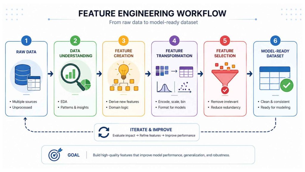
Feature engineering is not a step-by-step linear process, but rather an iterative and cyclical workflow.
3.1. Understand the Raw Data
Before any transformation, practitioners must deeply understand the data, its structure, distributions, missing value patterns, data types, and domain context. This stage involves exploratory data analysis (EDA): summary statistics, correlation matrices, visualizations, and discussions with domain experts. A common mistake here is skipping EDA and jumping straight to transformation, which leads to engineering features that are technically correct but semantically wrong.
3.2. Create New Features from Existing Data
New features are derived from existing columns through domain-driven logic or observed data patterns. A logistics model might derive delivery_delay_days by subtracting expected from actual delivery date. A banking model might create debt_to_income_ratio from two separate columns. Synthetic features built from combinations of existing variables often encode real-world relationships that raw columns do not individually represent.
3.3. Transform and Encode Features
Raw features must be converted into formats that algorithms can process. Categorical variables need to be encoded (one-hot, ordinal, or target encoding). Continuous variables may need to be scaled, log-transformed, or binned. Date columns are decomposed into time-based sub-features. The correct transformation depends on both the data distribution and the model’s assumptions, tree-based models are invariant to monotonic transformations, while linear and distance-based models are not.
3.4. Build Reusable Feature Pipelines
Production ML systems require that features computed during training are computed identically at inference time. This means feature logic must be encapsulated in reusable pipelines, not ad hoc scripts. Frameworks such as scikit-learn’s Pipeline, Apache Spark MLlib, and Feast (a feature store) enforce this consistency and reduce the risk of training-serving skew.
3.5. Select the Most Relevant Features
Not all engineered features add value. Feature selection removes redundant, irrelevant, or highly correlated features using filter methods (correlation, mutual information), wrapper methods (recursive feature elimination), or embedded methods (LASSO regularization, tree-based importance scores). Overly wide feature sets increase training time, risk overfitting, and reduce interpretability.
3.6. Validate Feature Impact on Model Performance
Features must be validated against model performance metrics, accuracy, AUC-ROC, RMSE, or others relevant to the task. Ablation studies (removing one feature at a time) and permutation importance analyses reveal which features drive performance. This step closes the loop: validation results inform the next round of feature creation and transformation.
4. Common Feature Engineering Techniques
Before diving into specific techniques, it is important to understand that feature engineering is not a single fixed step but a collection of practical methods used to improve how raw data is represented for machine learning models.
Different types of data, such as numerical values, categories, timestamps, or text, require different transformation strategies.
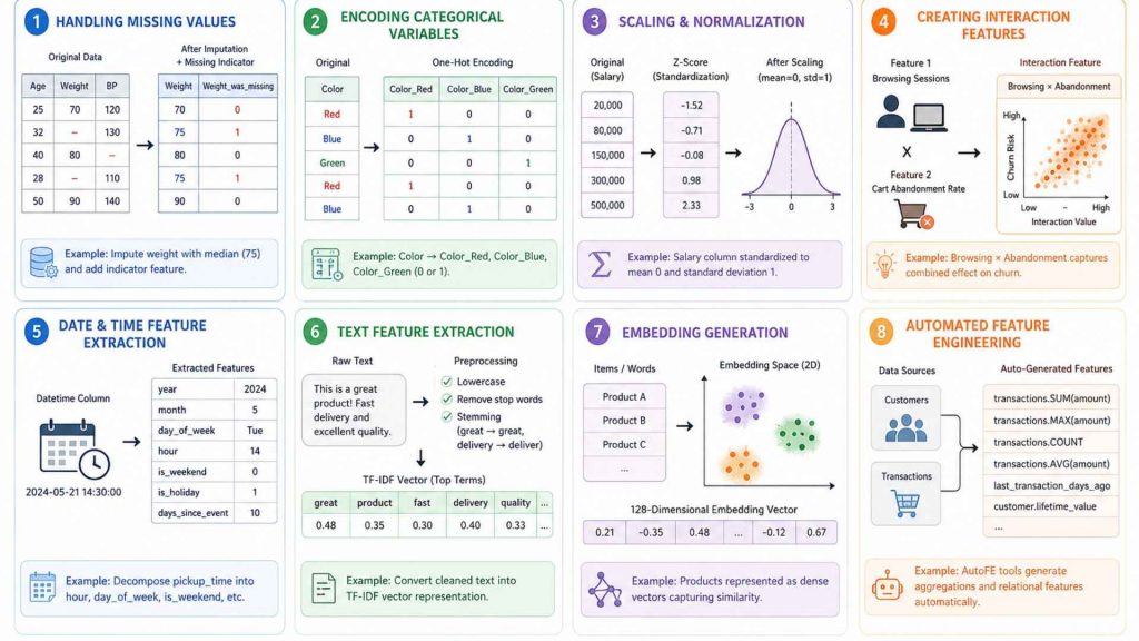
4.1. Handling Missing Values
Missing data is nearly universal in real-world datasets. The wrong imputation strategy can introduce bias or mask important patterns. Mean/median imputation is common for numerical features; mode imputation works for categorical ones. More sophisticated approaches include KNN imputation, model-based imputation, or treating missingness as a signal by adding a binary is_missing indicator feature alongside the imputed value.
Example: In a healthcare dataset, patient weight has 15% missing values. Rather than dropping those rows, the team imputes with the median and adds a binary feature weight_was_missing = 1. The model learns that missingness itself correlates with certain diagnoses.
4.2. Encoding Categorical Variables
Machine learning models require numerical inputs. Categorical variables, such as product category, country, or user type, must be encoded. One-hot encoding creates binary columns for each category (suitable for nominal variables with low cardinality). Ordinal encoding maps categories to ordered integers (suitable for ranked variables like Low/Medium/High). Target encoding replaces categories with the mean target value per category, powerful but prone to data leakage if not applied within cross-validation folds.
Example: A column Color with values Red, Blue, Green becomes three binary columns: Color_Red, Color_Blue, Color_Green, each containing 0 or 1.
4.3. Scaling and Normalization
Features measured on different scales can cause gradient-based and distance-based models to behave poorly. Min-max scaling compresses values to a [0, 1] range, preserving relative distances but amplifying outlier influence. Z-score standardization rescales features to mean 0 and standard deviation 1, making it suitable for PCA and LDA. Log transformation handles right-skewed distributions by compressing the tail. Tree-based models are generally scale-invariant; linear and neural network models are not.
Example: A salary column ranges from 20,000 to 500,000. After z-score standardization, values are centered around 0 with a standard deviation of 1, preventing salary from dominating gradient updates in a logistic regression model.
4.4 Creating Interaction Features
Interaction features capture the combined effect of two or more variables that are not captured by either individually. They are particularly valuable when the relationship between a predictor and the target depends on the value of another predictor, a pattern that linear models cannot learn without explicit interaction terms.
Example: In an e-commerce churn model, neither browsing_sessions nor cart_abandonment_rate alone predicts churn as well as their product: browsing_sessions × cart_abandonment_rate. Users who browse frequently but abandon carts consistently are far more likely to churn.
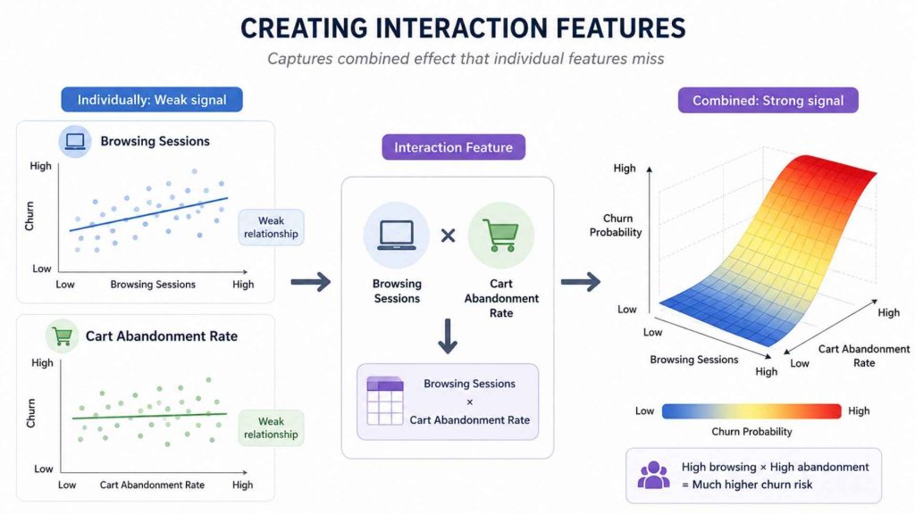
Instead of analyzing variables in isolation, interaction features highlight how they synergize to create a collective impact.
4.5 Date and Time Feature Extraction
Raw datetime columns are opaque to most models. Decomposing them into interpretable sub-features unlocks temporal patterns: hour_of_day, day_of_week, week_of_year, month, quarter, is_weekend, is_holiday, days_since_event. For time series problems, lag features (value at t-1, t-7) and rolling aggregates (7-day average, 30-day max) are especially powerful.
Example: A ride-sharing demand model decomposes pickup_time into hour (peak vs. off-peak), day_of_week (weekday vs. weekend), and is_public_holiday, capturing the three strongest temporal demand drivers.
4.6 Text Feature Extraction
Text data must be converted into numerical representations. Classical approaches include Bag of Words (count-based term frequency vectors), TF-IDF (term frequency adjusted by inverse document frequency to down-weight common words), and n-gram features (sequences of consecutive words). Preprocessing steps, lowercasing, stop word removal, stemming or lemmatization, reduce vocabulary noise before vectorization.
Example: A sentiment analysis model processes customer reviews by removing stop words, applying stemming (running → run), and converting the cleaned text into a TF-IDF matrix where each row is a review and each column is a weighted term frequency.
4.7 Embedding Generation
Dense vector embeddings represent words, entities, or items in a continuous vector space where semantic similarity corresponds to geometric proximity. Word2Vec, GloVe, and FastText produce word embeddings; transformer models (BERT, GPT) produce context-aware sentence embeddings. Recommendation systems use collaborative filtering embeddings to represent users and items. These dense representations carry far more information per dimension than sparse one-hot or TF-IDF vectors.
Example: A product recommendation system represents each product as a 128-dimensional embedding trained on co-purchase history. Products frequently bought together cluster in the embedding space, enabling similarity-based recommendations.
4.8 Automated Feature Engineering
Manual feature engineering is time-consuming and requires significant domain knowledge. Automated feature engineering (AutoFE) tools generate candidate features programmatically from raw datasets, using deep feature synthesis (DFS), genetic programming, or other search strategies. Libraries such as Featuretools and tsflex handle structured and time series data respectively. AutoFE is increasingly integrated into broader AutoML frameworks that automate the full ML pipeline from preprocessing to model selection.
Example: Featuretools traverses relationships between a customer table and a transactions table, automatically generating features like transactions.SUM(amount), transactions.MAX(amount), and transactions.COUNT, reducing hours of manual work to minutes.
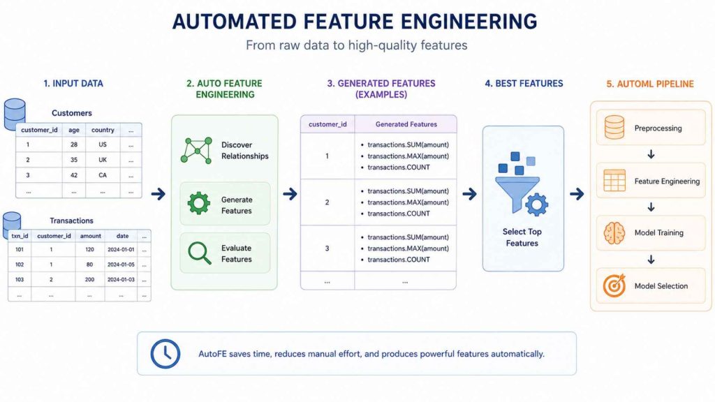
Automated Feature Engineering (AutoFE) tools like Featuretools and tsflex replace time-consuming manual processes.
5. Feature Engineering vs Feature Selection vs Feature Extraction
Feature engineering, feature selection, and feature extraction are often used interchangeably, but they represent different processes in the ML workflow with distinct roles and purposes.
| Criteria | Feature Engineering | Feature Selection | Feature Extraction |
| Definition | Creating, transforming, or modifying features from raw data | Selecting a relevant subset of existing features | Transforming original features into a new feature space |
| Main purpose | Improve the quality and representativeness of features | Reduce dimensionality and remove redundant variables | Compress information into lower-dimensional representations |
| Scope | Expands or reshapes the feature space | Narrows the feature set | Reconstructs features into new representations |
| Key tasks | Encoding, scaling, feature creation, interaction terms, embeddings | Correlation filtering, RFE, LASSO, mutual information | PCA, SVD, autoencoders, embeddings |
| When it happens | During the data preprocessing stage before model training | After feature engineering, before or during training | Before training, typically for high-dimensional data (tabular, text, images) |
| Impact on model performance | Adds informative signals that improve learning | Reduces overfitting and improves generalization | Reduces dimensionality while preserving key information |
| Example | Decomposing timestamp into hour_of_day and is_weekend | Removing one of two highly correlated features | Applying PCA to reduce 100 financial indicators into 10 principal components |
6. Feature Engineering Use Cases
Feature engineering powers a wide range of real-world machine learning applications, where carefully designed features transform raw data into actionable signals that drive accurate predictions and meaningful business decisions.
6.1. Fraud detection
Industry: Banking & Financial Services
Raw transaction data, card number, amount, timestamp, merchant ID, carries almost no individual fraud signal. Feature engineering surfaces the patterns that matter: transaction velocity (number of charges in the past 60 minutes), deviation from a customer’s historical spending baseline, and time-gap between geographically distant transactions. These behavioral constructs are what separates a model that flags fraud from one that misses it.
The IEEE-CIS fraud dataset showed that a multimodal feature engineering framework combined with LightGBM achieved an AUC of 0.968, surpassing strong baselines by 12.6%, while maintaining a false positive rate of just 0.7% and inference latency of 3ms. Separately, research confirmed that AI-based fraud detection models achieve accuracy rates between 87–96.8% in real-world deployments, significantly outperforming traditional rule-based systems which averaged only 37.8% accuracy.
Example: A bank engineers tx_count_1h (transactions in the past hour per card) and amount_zscore_90d (standard deviation from the customer’s 90-day average). A transaction with both values spiking simultaneously becomes a high-priority fraud alert, invisible to any model working on raw rows.
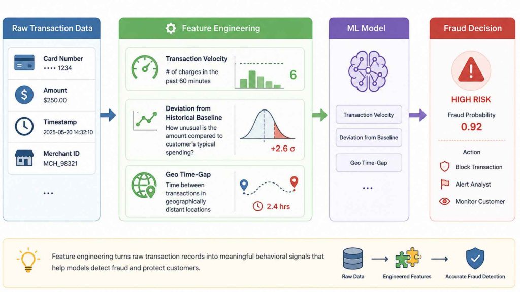
Raw transaction data has limited fraud signal, but feature engineering reveals key behavioral patterns that improve fraud detection.
6.2. Customer segmentation
Industry: Retail, E-commerce, Banking
Segmentation models need compact, comparable representations of customer behavior, not raw transaction logs. RFM feature engineering compresses an entire purchase history into three engineered columns: Recency (days since last purchase), Frequency (purchase count over a defined window), and Monetary value (total spend). From these three features, K-means clustering reliably separates loyal high-value customers from at-risk and one-time buyers, a segmentation directly actionable for CRM campaigns.
A study applying RFM features to Indian retail transaction data, combined with XGBoost, achieved an accuracy of 92.40%, precision of 92.27%, and an AUC score of 97.39% in predicting customer repurchase behavior, using only engineered features with no raw columns fed to the model. Teams iterating through feature variants like these benefit from a notebook environment where EDA, feature creation, and experiment comparison happen in the same workspace.
Example: From millions of raw order rows, three features are derived per customer. Customers with low recency, high frequency, and high monetary value are identified as the loyalty cohort; those with high recency and zero repeats are routed to win-back campaigns.
6.3. Recommendation systems
Industry: Streaming, E-commerce, Media
Recommendation systems are only as good as the features representing users and items. Raw interaction logs, clicks, watch time, purchases, must be engineered into dense behavioral embeddings that encode preference, context, and recency. The YouTube recommendation system employs a complex feature engineering framework that processes billions of user interactions across millions of items; at Netflix, the system incorporates diverse user features including viewing history, search patterns, and time-of-day preferences.
The 2025 RecSys Challenge winner results made the role of feature engineering explicit: the 4th-place solution integrated a sequential encoder, a graph neural network, a deep cross network, and performance-critical feature engineering to build user behavioral profiles generalizing across six downstream prediction tasks, churn, category preference, and SKU-level recommendations simultaneously.
Example: A streaming platform engineers a genre_affinity_score per user as the recency-weighted average of genre embeddings from the last 30 completed titles. Combined with a completion_rate feature, this single engineered signal outperforms raw watch-count features as a ranking input.
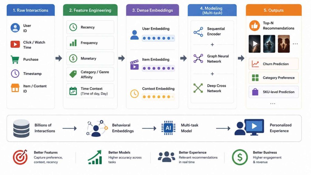
Top recommendation systems rely on transforming raw logs into behavioral embeddings to accurately capture user preferences and context.
6.4. Demand forecasting
Industry: Retail, Automotive, Supply Chain
Demand forecasting lives and dies on temporal feature engineering. A raw daily sales figure tells a model nothing about seasonality, promotions, or lifecycle decay. Engineered features do: lag variables (sales_t7, sales_t14), rolling averages (7-day, 28-day), calendar signals (is_holiday, days_until_promo), and external indicators (weather, fuel price) capture the contextual patterns that drive actual demand.
A 2025 Scientific Reports study on automotive spare-part demand forecasting across 1,709 part numbers showed that feature engineering capturing lagged demand, replacement intensity, and vehicle dropout dynamics allowed a Random Forest model to achieve a forecasting accuracy of 4.36% SMAPE over an 8-year horizon. An ablation study confirmed that removing lag and decay features degraded accuracy substantially, validating that the features, not the model, drove performance.
Example: A retailer engineers rolling_7d_avg_sales, is_public_holiday, and a lag feature sales_t7 from raw POS data. A LightGBM model on these features reduces stockout events for high-velocity SKUs compared to a baseline trained on raw daily counts alone.
6.5. Natural language processing
Industry: Healthcare, Customer Service, Legal, Media
NLP models depend almost entirely on how text is represented as features. Classical pipelines use TF-IDF vectors, n-gram counts, and handcrafted lexical signals. Modern pipelines use contextual embeddings from transformer models, BERT, RoBERTa, domain-specific variants, that encode semantics, syntax, and domain vocabulary in dense vectors. The choice of text representation is itself a feature engineering decision with direct performance consequences.
In healthcare, Alsentzer et al. adapted BERT to clinical notes, releasing ClinicalBERT, which showed significant improvements in healthcare NLP tasks including clinical natural language inference. A systematic evaluation comparing TF-IDF, Doc2Vec, and BERT on surgical operative notes found that combining BERT embeddings with handcrafted domain features, such as a boolean contains_procedure_keyword, produced more robust classification on short, ambiguous notes than either approach alone.
Example: A health insurer processing claim dispute letters engineers three feature types: a ClinicalBERT sentence embedding, a TF-IDF score for escalation terms, and a binary contains_legal_reference flag. The combined feature set routes the majority of letters to the correct handling queue without human review, versus far fewer with TF-IDF alone.
6.6. Machine learning experimentation and model development
Industry: Cross-industry
Feature engineering is not a one-pass task, it is an iteration loop. Data scientists explore raw datasets, hypothesize transformations, rerun training, compare metric deltas, and repeat. This workflow requires a unified environment where EDA, feature authoring, training jobs, and experiment tracking happen without switching tools. Fragmented setups, a local notebook here, a remote training script there, results scattered across email, slow iteration and make experiments hard to reproduce.
Example: A credit scoring team iterates through 12 feature variants in three days, testing one-hot vs. target encoding for employment_type, comparing 30-day vs. 90-day lag windows for payment_history, logging AUC-ROC per configuration, with all results traceable and shareable within the same notebook environment.
For ML teams that need a managed, consistent workspace for this process, AI Notebook provides an environment where data scientists can explore datasets interactively, write and test feature pipelines, run experiments, and compare model performance, all within one collaborative platform that keeps experiments reproducible from first hypothesis to final model.
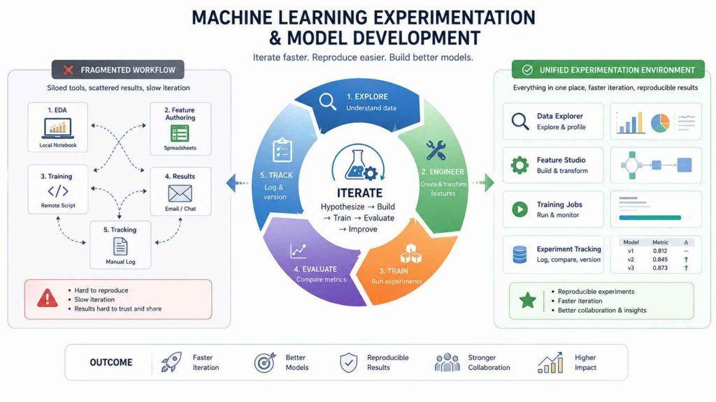
Feature engineering is an iterative loop that requires a single, unified environment to prevent fragmented setups.
7. Feature Engineering in Modern Machine Learning Workflows
As machine learning systems move from research prototypes to large-scale production environments, feature engineering has evolved from manual preprocessing into a fully integrated component of modern ML infrastructure.
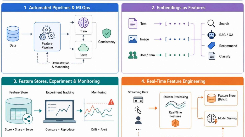
7.1. Automated Feature Pipelines and MLOps
In production ML systems, feature engineering cannot remain a collection of ad hoc scripts. Reusable feature pipelines encapsulate transformation logic in versioned, testable code that runs identically during training and inference. Orchestration platforms such as Apache Airflow, Prefect, and Kubeflow Pipelines schedule and monitor these pipelines as part of broader MLOps workflows.
A critical concern in MLOps is training-serving consistency: the features a model saw during training must be computed using the exact same logic at prediction time. Inconsistencies between training and serving pipelines, often called training-serving skew, are a leading cause of degraded production model performance that is difficult to diagnose.
>> Explore more: MLOps vs DevOps: Key Differences, Use Cases & How to Choose
7.2. Embedding-Based Features for AI Applications
Dense vector embeddings have become a foundational feature type in modern AI applications. Text embeddings from transformer models capture semantic similarity across documents, queries, and knowledge bases. Image embeddings from convolutional or vision transformer models represent visual content in compact, comparable vectors. In recommendation systems, collaborative filtering generates user and item embeddings that encode behavioral similarity.
For LLM-based applications, retrieval-augmented generation (RAG), semantic search, document classification, embedding generation is itself a feature engineering step: transforming raw text into vector representations that a retrieval system or classifier can operate on.
7.3. Feature Stores, Experimentation, and Monitoring
As organizations scale their ML programs, feature stores, centralized repositories for engineered features, have emerged as essential infrastructure. Feature stores such as Feast, Tecton, and Hopsworks enable feature versioning (ensuring reproducibility), feature sharing across teams (reducing duplication), and consistent serving between training and production environments.
Experiment tracking platforms (MLflow, Weights & Biases) log which features were used in each experiment alongside model metrics, making it possible to reproduce results and compare feature variants systematically. Feature monitoring, tracking feature distributions over time and detecting drift, ensures that features computed on live data remain consistent with those seen during training.
7.4. Real-Time Feature Engineering
Many high-value ML applications require features computed in real time, fraud detection at transaction swipe, dynamic pricing at page load, personalized ranking at search query. Real-time feature engineering involves streaming computation (Apache Kafka, Apache Flink) that ingests raw events, applies feature logic, and serves computed features to models within milliseconds.
Real-time features are often combined with precomputed batch features stored in a feature store, creating a hybrid feature architecture that balances recency (real-time signals) with richness (historical aggregates).
Enhancing model performance through advanced feature engineering methodologies within contemporary machine learning production pipelines.
8. Feature Engineering Challenges
Despite its critical role in building high-performing machine learning systems, feature engineering also introduces a range of practical challenges that span data understanding, implementation complexity, and production reliability. These challenges often become more pronounced as:
- Requires domain knowledge: Knowing which features to engineer requires understanding the problem domain. A data scientist without retail industry context may miss the significance of a promotional calendar feature.
- Time-consuming and iterative: Good features rarely emerge from the first attempt. The iterative nature of feature engineering, hypothesize, transform, validate, refine, can consume the majority of an ML project’s timeline.
- Risk of data leakage: Features computed using information from the test set or future data contaminate model evaluation. Target encoding applied outside cross-validation folds and lag features computed without proper time ordering are common leakage sources.
- Feature redundancy and overfitting: Generating too many features increases dimensionality, introduces noise, and risks overfitting, especially with limited training data. Feature selection and regularization become essential safeguards.
- Depends heavily on data quality: Feature engineering cannot compensate for fundamentally broken data. Systematic measurement errors, inconsistent category labels, and biased sampling propagate through engineered features into model predictions.
- Training-production consistency: Every transformation applied during training must be replicated precisely in production. Undocumented preprocessing steps, hardcoded imputation values, and environment-specific library versions all introduce risk.
This last challenge, maintaining consistent feature pipelines across development and production, is where infrastructure matters as much as engineering skill. ML teams that need a containerized environment to run feature engineering pipelines, training jobs, and production workflows consistently can use GPU Container. It provides isolated, reproducible compute environments that eliminate the ‘it worked on my machine’ problem, ensuring that feature logic runs identically from development through deployment.

Rent high-end GPUs for scaling your AI faster (Source: FPT AI Factory)
9. FAQs
9.1. What is feature engineering in simple terms?
Feature engineering is the process of transforming raw data into inputs that a machine learning model can understand and learn from. Think of it as translating messy, real-world information, timestamps, text, categories, missing values, into a clean, numerical language that algorithms speak. Without feature engineering, even a powerful model will struggle to find signal in unprocessed data.
9.2. What is the difference between feature engineering and feature selection?
Feature engineering creates or transforms features, it expands and reshapes what the model has to work with. Feature selection chooses which features to keep, it narrows the feature set by removing redundant or irrelevant variables. In practice, feature engineering comes first (generating candidates), and feature selection follows (pruning them). Both contribute to better model performance, but through opposite mechanisms: one adds signal, the other reduces noise.
9.3. Is feature engineering needed for deep learning?
Deep learning models can learn hierarchical feature representations automatically from raw data, particularly for images, audio, and text, where convolutional and transformer architectures extract features without manual engineering. However, feature engineering remains relevant even in deep learning contexts: structured tabular data still benefits significantly from domain-driven feature construction; input normalization and encoding remain necessary; and hybrid approaches that combine engineered features with learned representations frequently outperform either approach alone.
9.4. What are common feature engineering techniques?
The most widely used techniques include: handling missing values (imputation with indicator flags), encoding categorical variables (one-hot, ordinal, target encoding), scaling and normalization (min-max, z-score), creating interaction features (products or ratios of existing variables), date and time decomposition (hour, day_of_week, is_holiday), text feature extraction (TF-IDF, bag of words), embedding generation (Word2Vec, BERT), and automated feature engineering (Featuretools, AutoML pipelines). The right combination depends on the data type, model architecture, and problem domain.
Feature engineering remains a core step in any machine learning workflow. Even with advanced models such as deep learning or gradient boosting, the way raw data is transformed into features often has a greater impact on model performance than the algorithm itself.
Across applications like fraud detection, recommendation systems, demand forecasting, and NLP, one consistent pattern stands out: better features lead to more stable, accurate, and interpretable models. At the same time, feature engineering is closely tied to experimentation and infrastructure, where teams need a reliable environment to test ideas, run training jobs, and compare results in a reproducible way.
For new users, FPT AI Factory also offers a Starter Plan with $100 credits, allowing individuals and teams to explore AI Notebook, GPU compute, and experiment workflows before scaling into production. For enterprise requirements, tailored options are available with dedicated support, secure infrastructure, and flexible deployment capabilities. Contact FPT AI Factory for more details now!
Contact Information:
- Hotline: 1900 638 399
- Email: support@fptcloud.com
Explore more