
What is learning rate, and why does it play such a decisive role in the success of any machine learning model? Understanding learning rate helps practitioners control training speed, avoid common pitfalls like overshooting or slow convergence, and ultimately build more accurate, efficient AI systems. At FPT AI Factory, we provide cutting-edge AI solutions that empower teams to master every aspect of model training, from tuning hyperparameters to deploying production-ready models at scale.
1. What Is Learning Rate?
Learning rate is a hyperparameter that determines the size of each weight update during training. In gradient-based optimization, weights are updated according to the formula:
[
w_{t+1} = w_t – \eta \nabla L(w_t)
]
where (w_t) is the current weight, (\nabla L(w_t)) is the gradient of the loss function, and (\eta) is the learning rate. The learning rate directly scales the update step: a larger (\eta) produces larger movements in the parameter space, while a smaller (\eta) results in more gradual adjustments.
Intuitively, learning rate can be compared to the step size taken when walking downhill toward the lowest point of a valley (the minimum loss). If the steps are too large, the model may overshoot the optimum, oscillate around it, or even diverge. If the steps are too small, training becomes slow and may stall on flat regions of the loss landscape. Therefore, choosing an appropriate learning rate is critical for balancing training speed, stability, and final model performance.
In large-scale GPT training, Li et al. found that increasing batch size and learning rate can improve training efficiency, but pushing them too far may lead to instability and failed training runs.
A simple way to understand this is to imagine walking down a mountain toward the lowest point in a valley, which represents the optimal model parameters. If the learning rate is too high, you may take huge jumps, overshoot the valley, and keep bouncing around without reaching the bottom. If the learning rate is too low, you take tiny steps and need a very long time to get there. A well-chosen learning rate allows you to reach the valley efficiently while maintaining stability.
To address instability at large scales, Li et al. proposed the Sequence Length Warmup method, which gradually increases the training sequence length during early training. This approach enabled the use of much larger batch sizes and learning rates without causing divergence, reducing both the number of training tokens and overall wall-clock training time while preserving strong zero-shot performance.

Learning rate directly shapes three core training outcomes
2. How Does Learning Rate Work?
Learning rate operates through a repeating four-step cycle during model training. Each iteration refines the model’s weights until the loss reaches its minimum.
2.1 Loss calculation
At the start of each cycle, a loss function measures the gap between the model’s predictions and the actual target values. The result is a single number representing how wrong the model currently is. Minimizing this loss by adjusting model parameters is the central goal of the entire training process. A smaller loss means the model’s outputs are closer to the ground truth.
For example, in MNIST digit classification, a model predicts one of 10 digit classes from 28×28 grayscale images. Cross-entropy loss is commonly used to compare the model’s predicted probabilities with the correct digit label, so a lower loss means the model is recognizing handwritten digits more accurately.
2.2 Gradient calculation
Once the loss is known, the gradient, a vector pointing in the direction of steepest ascent on the loss surface, is computed with respect to each weight. Since the objective is to reduce loss rather than increase it, the optimizer moves in the exact opposite direction. The weight update is computed by stepping in the opposite direction of the cost gradient, where η (eta) represents the learning rate that scales how large that step will be.
For instance, TensorFlow uses automatic differentiation to record operations during the forward pass and compute gradients during the backward pass. For example, if a model processes MNIST images with 784 pixel inputs, TensorFlow can calculate gradients for the weights connected to those inputs without manually deriving each partial derivative.
2.3 Weight update size
Each parameter gets updated by a constant value, the learning rate, weighted by how much that parameter contributes to minimizing the loss, which is its gradient. In practice, this means that the model first decides the step size, then the gradient tells it the relative impact of moving each weight. The model multiplies the gradient by the learning rate to determine the new weight and bias values for the next iteration.
In a real case, TensorFlow’s optimizer guide shows gradient descent updating each variable by subtracting learning_rate × gradient. In its sample loss function, the global minimum occurs at x = -9/8, and different learning rates affect how quickly or safely the optimizer moves toward that minimum.
2.4 Repeated training iterations
Steps 2 and 3 are repeated until the loss function converges to a minimum or a predefined stopping criterion is met. Over hundreds or thousands of iterations, weights shift steadily toward values that minimize prediction error. When a model can no longer be improved through further training, it is said to have reached convergence, the final goal of the entire optimization loop.
In the TensorFlow MNIST tutorial, training uses batches of images and labels to repeatedly update weights and biases. The guide notes that a batch size such as 128 images can give a gradient that better represents different examples and helps the model converge faster than updating from only one image at a time.
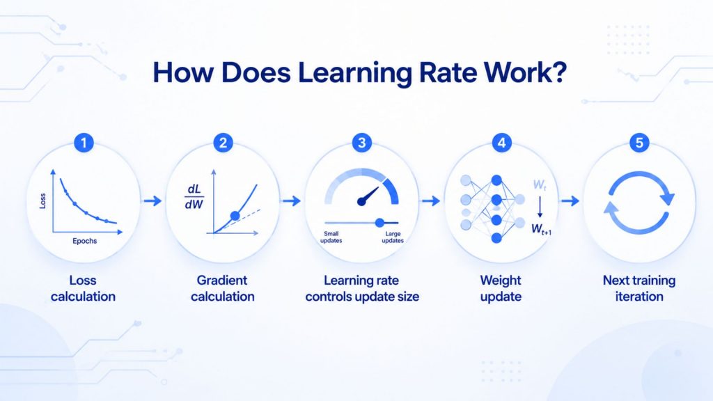
Learning rate operates through a repeating four-step cycle during model training
3. Why Learning Rate Matters in Machine Learning?
Learning rate is one of the most important hyperparameters because it controls how much a model changes after each training update. A good learning rate helps the model learn efficiently, while a poor value can make training unstable, slow, or inaccurate.
- Training stability: A suitable learning rate helps the model update weights smoothly, reducing unstable loss curves, noisy optimization, or failed convergence during training.
- Faster convergence: When the learning rate is well-tuned, the model can reach a useful loss level faster without wasting too many training epochs.
- Avoiding overshooting: If the learning rate is too high, updates may jump past the optimal point, causing the loss to oscillate instead of improving.
- Preventing slow learning: If the learning rate is too low, training may progress very slowly and require far more time, data passes, and computing resources.
- Impact on model accuracy: The learning rate directly affects how well the model learns patterns, as poor updates can lead to underfitting or unstable final performance.
- Affects GPU training efficiency: Better learning rate choices can reduce unnecessary epochs, helping teams use GPU time more efficiently during deep learning experiments.

Learning rate is one of the most important hyperparameters
4. Common Types of Learning Rate Strategies
No single learning rate strategy fits all problems. Each method is designed to address different limitations in the optimization process, ranging from simplicity in implementation to the ability to adapt dynamically to individual parameters.
4.1 Constant learning rate
Constant learning rate serves as the default baseline strategy in many deep learning frameworks such as Caffe, TensorFlow, and Torch, where a fixed learning rate value is maintained throughout the entire training process. Its greatest advantage is simplicity and ease of implementation, requiring no additional scheduling configuration. However, its lack of adaptability may hinder optimization in complex scenarios where the ideal learning rate changes over time.
Training a simple MLP on the MNIST dataset with a fixed lr = 0.01 over 20 epochs typically yields stable convergence, but remains suboptimal in terms of speed during the final stages.
4.2 Step decay
Step decay is one of the most widely used learning rate adjustment methods, built on the core idea of starting with a relatively high learning rate and then reducing it by a set factor at predefined epoch milestones. This approach enables the model to learn quickly in the early stages and make finer, more precise updates as it approaches convergence. The main drawback is that parameters such as the decay factor and step interval must be determined empirically, requiring additional manual tuning effort.
In PyTorch, StepLR(optimizer, step_size=10, gamma=0.1) reduces the learning rate by a factor of 10 every 10 epochs. This approach is widely used when training ResNet on ImageNet.
4.3 Exponential decay
Exponential decay reduces the learning rate smoothly and continuously over time, supporting a more stable and efficient optimization process compared to step-based approaches. Rather than dropping abruptly at fixed milestones, the learning rate is multiplied by a constant factor smaller than 1 after each update step. However, an improperly chosen decay rate can cause the learning rate to decrease too aggressively, significantly slowing convergence and extending total training time.
In TensorFlow/Keras, ExponentialDecay(initial_learning_rate=0.1, decay_steps=1000, decay_rate=0.96) reduces the learning rate by 4% every 1,000 steps, commonly applied when training CNNs on MNIST or CIFAR-10.
4.4 Cosine annealing
Cosine annealing adjusts the learning rate along a cosine curve, gradually reducing it over each cycle in a smooth pattern that helps stabilize training and avoid oscillation around suboptimal solutions. A notable feature is the warm restart mechanism, where the learning rate resets to its initial value at the start of each new cycle to escape poor convergence regions. This strategy is widely adopted in training large language models such as GPT and LLaMA.
When fine-tuning BERT, the standard learning rate schedule typically combines a linear warmup phase with cosine annealing decay to stabilize training and improve generalization.
4.5 Adaptive learning rates (Adam, RMSProp)
With adaptive methods such as Adam and RMSProp, the learning rate is adjusted individually for each parameter rather than applying a single global value, ensuring convergence even when the input data is not linearly separable. Adam tracks exponentially weighted moving averages of both the gradient and its squared values, allowing it to adapt effectively across virtually any neural network architecture.
In PyTorch, optim.Adam(model.parameters(), lr=0.001, betas=(0.9, 0.999)) is the recommended default configuration for most deep learning tasks, spanning both NLP and computer vision.
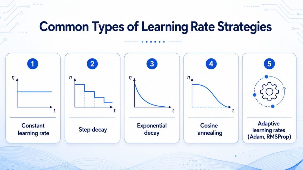
Each method is designed to address different limitations in the optimization process
5. Common Learning Rate Problems During Training
Choosing an inappropriate learning rate does not simply slow down the training process, it directly compromises the effectiveness of optimization, convergence behavior, and the overall performance of the model.
5.1 Learning rate too high
When the learning rate is set too high, the optimization process tends to jump over minima rather than converging toward them, resulting in divergence or uncontrolled oscillation across the loss landscape. Weight updates become excessively large, causing the model to repeatedly overshoot the optimal region and fail to stabilize at a good solution.
In more severe cases, an overly high learning rate can lead to overfitting, where the model captures noise in the training data rather than meaningful underlying patterns.
5.2 Learning rate too low
When the learning rate is too low, convergence becomes extremely slow, and the model risks getting trapped in undesirable local minima without making further progress. Although the model may eventually reach a solution, the significantly larger number of epochs required drives up both computational cost and training time. Furthermore, an excessively small learning rate can result in underfitting, leaving the model unable to learn the important patterns present in the data.
5.3 Training instability and oscillation
A poorly tuned learning rate can produce oscillations in the loss curve, destabilizing the optimization process and preventing the model from reliably reaching a good solution. This instability typically manifests as erratic fluctuations in the loss across epochs rather than a steady downward trend. When combined with high-norm gradients, the model may continuously shift toward worse regions of the parameter space, creating a diverging cycle instead of converging.
5.4 Overfitting and poor convergence
A learning rate that is too high can cause the model to overshoot the optimal point and diverge, while one that is too low leads to extremely slow convergence or the model becoming trapped in a local minimum.
Beyond training speed, poor convergence often reflects a deeper issue where the optimizer settles at a saddle point or local minimum rather than a global one. Convergence alone does not guarantee an optimal solution, as the outcome depends on multiple factors, including data quality, network architecture, and the chosen hyperparameters.
5.5. Gradient explosion or vanishing
When the learning rate is excessively high, weight update magnitudes become extreme, driving the network’s parameters to diverge rather than converge, often visible as a rapidly increasing or wildly oscillating loss during training.
In the opposite direction, vanishing gradients occur when gradients become extremely small during backpropagation, causing earlier layers to learn very slowly or stop learning entirely. Both problems are particularly severe in deep neural networks, where gradient amplification or attenuation accumulates across many layers.
5.6. Learning rate tuning and experimentation
Selecting an appropriate learning rate still relies heavily on trial and error, accumulated experience, or tools such as a learning rate finder to identify a suitable starting value. Two widely used hyperparameter search strategies are Grid Search and Random Search, which proves more efficient when the parameter space is large.
Research by Bergstra and Bengio (2012), published in the Journal of Machine Learning Research, demonstrated that Random Search is generally more efficient than Grid Search, especially as the number of hyperparameters to tune increases.
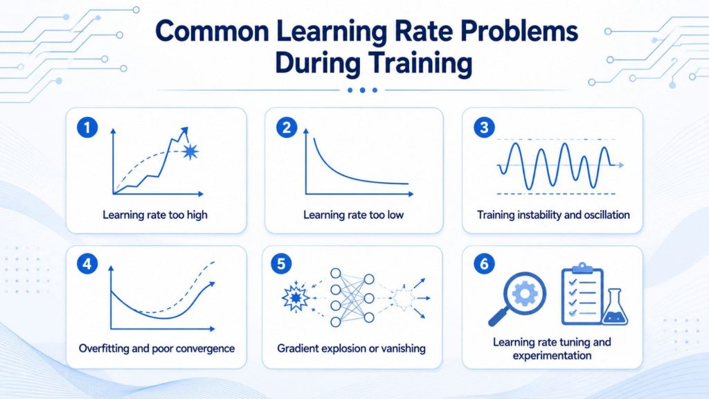
Choosing an inappropriate learning rate does not simply slow down the training process
6. Learning Rate Finder
Choosing an appropriate learning rate is often challenging because values that are too high can cause training instability, while values that are too low can significantly slow convergence. To address this issue, researchers and practitioners commonly use a Learning Rate Finder, a technique that automatically explores a range of learning rates before full training begins.
The basic idea is to start with a very small learning rate and gradually increase it over several mini-batches while monitoring the training loss. As the learning rate increases, the loss typically decreases at first, reaches a stable region, and then starts increasing sharply when the learning rate becomes too large. The optimal learning rate is usually selected from the region where the loss is decreasing rapidly but remains stable.
A useful analogy is tuning the speed of a car before a long journey. Driving too slowly wastes time, while driving too fast increases the risk of losing control. A Learning Rate Finder helps identify the fastest safe speed, allowing the model to learn efficiently without becoming unstable.
For example, suppose a neural network is being trained for image classification. During a Learning Rate Finder test, the learning rate is gradually increased from 0.00001 to 1.0 while monitoring the training loss.
| Learning Rate | Training Loss Behavior |
| 0.00001 | Loss decreases very slowly |
| 0.0001 | Loss decreases steadily |
| 0.001 | Loss decreases rapidly |
| 0.01 | Loss reaches its steepest decline |
| 0.1 | Loss becomes unstable |
| 1.0 | Loss explodes and training diverges |
In this case, a learning rate around 0.001 – 0.01 would likely be selected because it provides fast learning without causing instability. This approach helps practitioners avoid extensive trial-and-error when tuning hyperparameters.
The Learning Rate Finder technique was introduced by Leslie Smith as the “Learning Rate Range Test.” The method gradually increases the learning rate over a short training run and identifies the region where the loss decreases most effectively before divergence occurs.
7. Learning Rate in Large AI Models
As AI models grow from millions to hundreds of billions of parameters, learning rate management becomes far more complex than in conventional deep learning settings. Each stage of a large model’s lifecycle different strategy for controlling the learning rate:
7.1 Training large language models
Training LLMs from scratch is feasible only with thousands of GPUs and substantial investment, making learning rate decisions far more consequential than in standard neural network training. At this scale, a misconfigured learning rate translates directly into wasted GPU-hours and financial cost. A scheduler combining warmup and annealing stages is considered essential for achieving optimal performance and generalization in language models.
For example, LLaMA 3.1 405B was trained using AdamW with a peak learning rate of 8e-5, a warmup phase of 8,000 steps, followed by cosine decay down to 1% of peak learning rate over 1.2 million training steps.
7.2 Distributed AI training
In distributed settings, the effective batch size grows proportionally with the number of GPU workers, requiring the learning rate to scale accordingly. The linear scaling rule allows large-batch distributed training to maintain accuracy comparable to single-device setups. A linear warmup is also necessary to stabilize the optimizer before reaching the full scaled learning rate. Without proper scaling, large-batch training tends to converge to sharp minima that generalize poorly.
At 512 GPUs with an effective batch size of 16,384, the naive single-GPU learning rate clearly fails, a problem addressed in the Facebook AI Research paper “Accurate, Large Minibatch SGD: Training ImageNet in 1 Hour.”
7.3 Fine-tuning foundation models
Fine-tuning a pretrained foundation model requires a lower and more carefully controlled learning rate to preserve the model’s existing general knowledge. For LoRA fine-tuning, starting with a learning rate of 2e-4 and applying a Warmup-Stable-Decay schedule is the recommended approach. AdamW remains the most widely used optimizer, with warmup steps set to around 10% of total training steps.
In LoRA experiments on LLaMA-based models, the best-performing AdamW configuration used lr=3e-4 with weight decay of 0.01, trained with batch size 128 via gradient accumulation on a single A100, completing in approximately 1.8 hours.
7.4 GPU resource optimization
Efficient GPU utilization and learning rate strategy are closely linked, since a poorly chosen learning rate wastes compute regardless of hardware quality. Mixed precision training in FP16 or BF16 delivers up to 16x faster matrix multiplication on A100 GPUs over FP32, while halving memory requirements, enabling larger batches within the same hardware budget. These memory savings allow larger effective batch sizes, which in turn require recalibrating the learning rate to maintain stable convergence.
NVIDIA benchmarks show a BERT training workload can complete in under a minute using 2,048 A100 GPUs, enabled by both hardware efficiency and carefully tuned learning rate schedules that keep training stable at extreme parallelism.
7.5. Learning rate schedulers for large-scale training
Modern large-scale training relies on multi-phase scheduling strategies rather than simple fixed or step-based approaches. The cosine learning rate schedule has become the dominant choice for training large language models and vision transformers. A newer approach, Warmup-Stable-Decay (WSD), is gaining traction, including warmup covers 1–2% of total steps, a stable plateau spans 60–80% for exploration, and a final decay phase of 10–25% allows the model to settle into an optimal solution.
Linear warmup followed by cosine decay is implemented via LambdaLR in PyTorch, with a peak learning rate of 3e-4, 10,000 warmup steps, and cosine decay over remaining steps, a configuration widely used in Hugging Face Transformers for LLM pretraining.
For enterprises looking to fine-tune LLMs at scale, managing learning rate schedules alongside GPU infrastructure is a non-trivial operational challenge. FPT AI Factory’s Model Fine-Tuning platform is purpose-built for these production-scale workflows, providing the GPU resources and tooling needed to run and iterate on large model fine-tuning efficiently.

Model Fine-Tuning platform is purpose-built for these production-scale workflows (Source: FPT AI Factory)
8. Learning Rate vs Batch Size vs Optimizer
These three factors do not operate in isolation, adjusting one typically requires reconsidering the others. The table below captures how they interact during model training and what practitioners should consider when tuning them together.
| Factor | What It Controls | Impact on Training | Example Consideration |
| Learning Rate | The step size taken at each parameter update during gradient descent | Directly determines convergence speed, stability, and final model quality. Too high causes divergence, too low causes slow or stuck training | Start with 1e-3 for Adam, reduce to 1e-5 when fine-tuning a pretrained model to avoid overwriting learned representations |
| Batch Size | The number of training samples used to compute each gradient estimate | Larger batches produce smoother, lower-variance gradients but risk converging to sharp minima that generalize poorly. Smaller batches add noise that can help escape local minima | Larger batches can utilize GPU parallel processing more effectively, but require more memory. The appropriate learning rate is closely tied to the noise level of the gradient estimate. |
| Optimizer | The algorithm that uses the gradient to update model parameters | Determines how adaptive the learning process is. SGD requires more manual tuning, while adaptive optimizers like Adam self-adjust per parameter | Adam is currently the most widely used optimizer in deep learning, combining Momentum and RMSProp to adapt effectively across virtually any neural network architecture. |
| Relationship between Learning Rate and Batch Size | Scaling one directly affects the other’s optimal value | Smaller batch sizes produce noisier gradient updates and require a lower learning rate for stability; larger batch sizes allow a higher learning rate due to more accurate gradient estimates. | The linear scaling rule suggests that when the batch size increases by k times, the learning rate should also scale proportionally, validated up to a batch size of 8,192 on ImageNet. |
| Relationship between Optimizer and Learning Rate Tuning | The optimizer type determines how sensitive training is to learning rate choice | For SGD-style optimizers, the optimal learning rate scales linearly with batch size. For Adam-style optimizers, this relationship is non-linear and requires separate empirical tuning. | AdamW with lr=3e-4 often works out of the box for most deep learning tasks. SGD with momentum requires careful, task-specific learning rate tuning |
| Practical Tuning Consideration | Finding the right combination of all three factors | No single combination works universally, each task, architecture, and dataset requires its own configuration | For LLM fine-tuning, a recommended starting point is AdamW with lr=2e-4, batch size 16–32, and a Warmup-Stable-Decay schedule, adjusting each component based on training loss behavior. |
9. FAQs
9.1 What happens if learning rate is too high?
If the learning rate is too high, the model may update its weights too aggressively and jump past the best solution instead of moving toward it. This can make the loss curve bounce, oscillate, or fail to converge, meaning the model cannot learn stable patterns from the data.
9.2 What is the best learning rate for neural networks?
There is no single best learning rate for all neural networks, because the right value depends on the dataset, model architecture, optimizer, batch size, and training objective. In practice, teams often test several values, use learning rate schedules, or rely on adaptive optimizers such as Adam and RMSprop.
9.3 Does learning rate affect accuracy?
Yes, learning rate can affect accuracy because it influences how well the model reaches a useful solution during training. A rate that is too low may learn too slowly or get stuck with weak performance, while a rate that is too high may prevent stable convergence. IBM notes that learning rate guides how effectively AI models learn from training data, which directly connects it to final model performance.
If you are ready to put these concepts into practice, FPT AI Factory offers everything you need to get started. FPT AI Factory offers a $100 free trial credit program for users to explore the platform. The credit is valid for 30 days and is allocated across the platform’s core services:
- $10 for GPU Container and $10 for GPU Virtual Machine
- $10 for AI Notebook and $70 for AI Inference & AI Studio
- Access to up to 5M tokens with Llama-3.3 and 20+ state-of-the-art models
For teams working on larger initiatives — such as fine-tuning foundation models, running distributed training pipelines, or deploying production-grade AI systems, FPT AI Factory provides tailored infrastructure and expert support. Reach out directly via the official contact form to discuss a solution built around your specific requirements.
In short, understanding what is learning rate is not just a theoretical exercise, it is a practical skill that compounds across every model you build. Whether you are training your first neural network or scaling a billion-parameter LLM, having the right tools and infrastructure behind you makes all the difference. Start with FPT AI Factory today and turn your understanding of learning rate into real, measurable results.
Contact Information:
- Hotline: 1900 638 399
- Email: support@fptcloud.com
Reference Articles
What is Fine-Tuning? An In-Depth Guide for When to Use
Key Evaluation Metrics in Machine Learning: Complete Guide
LLM Large Language Model Training & Fine Tuning Guide